Analyzing Patient Data

Objectives

• Explain what a library is and what libraries are used for.

• Import a Python library and use the functions it contains.

• Read tabular data from a file into a program.

• Select individual values and subsections from data.

• Perform operations on arrays of data.

Questions

• How can I process tabular data files in Python?

Scenario: A Miracle Arthiritis Inflamation Cure

Now that we’ve covered some Python basics, we’ll learn how to work with data.

Imagine we have a colleague “Dr. Maverick”. They’ve invented a new miracle drug that claims to cure arthritis inflammation flare-ups in only 3 weeks! Naturally, we want to see the clinical trial data, and after months of asking, they have finally provided it.

We’re going to use Python to analyze this data and decide if Dr. Maverick’s claims are true.

Data Format

The data sets are stored in comma-separated values (CSV) format:

• Each row holds information for a single patient.

• Columns represent successive days.

The first three rows of our first file look like this:

0,0,1,3,1,2,4,7,8,3,3,3,10,5,7,4,7,7,12,18,6,13,11,11,7,7,4,6,8,8,4,4,5,7,3,4,2,3,0,0
0,1,2,1,2,1,3,2,2,6,10,11,5,9,4,4,7,16,8,6,18,4,12,5,12,7,11,5,11,3,3,5,4,4,5,5,1,1,0,1
0,1,1,3,3,2,6,2,5,9,5,7,4,5,4,15,5,11,9,10,19,14,12,17,7,12,11,7,4,2,10,5,4,2,2,3,2,2,1,1

Each number represents the number of inflammation bouts that a particular patient experienced on a given day.

For example, value “6” at row 3 column 7 of the data set above means that the third patient was experiencing inflammation six times on the seventh day of the clinical study.

Loading data into Python

To begin processing the clinical trial inflammation data, we need to load it into Python. We can do that using a library called NumPy, which stands for “Numerical Python”. Libraries are collections of Python code written by other people that you can install and use.

In general, you should use NumPy you want to do fancy things with lots of numbers, especially if you have matrices or arrays. To tell Python that we’d like to start using NumPy, we need to import it[1]:

import numpy

Importing a library is like getting a piece of lab equipment out of a storage locker and setting it up on the bench. Libraries provide additional functionality to Python, much like a new piece of equipment adds functionality to a lab space. Just like in the lab, importing too many libraries can sometimes complicate and slow down your programs - so we only import what we need for each program.

Once we’ve imported the library, we can ask the library to read our data file for us:

numpy.loadtxt('data/inflammation-01.csv', delimiter=',')

array([[ 0.,  0.,  1., ...,  3.,  0.,  0.],
       [ 0.,  1.,  2., ...,  1.,  0.,  1.],
       [ 0.,  1.,  1., ...,  2.,  1.,  1.],
       ...,
       [ 0.,  1.,  1., ...,  1.,  1.,  1.],
       [ 0.,  0.,  0., ...,  0.,  2.,  0.],
       [ 0.,  0.,  1., ...,  1.,  1.,  0.]])

The expression numpy.loadtxt(...) is a function call that asks Python to run the function loadtxt of the numpy library. The dot notation (.) tells Python to look inside the numpy library and find the loadtxt function. When you see numpy.loadtxt, you can read it as “the loadtxt function that belongs to numpy”.

As an example, John Smith is the John that belongs to the Smith family. We could use the dot notation to write his name smith.john. smith is a container (family) that holds a lot of people, one of whom is john, just as numpy is a container (library) that holds a lot of functions, one of which is loadtxt.

numpy.loadtxt has two parameters: the name of the file we want to read and the delimiter that separates values on a line. These both need to be strings, so we put them in quotes.

Since we haven’t told it to do anything else with the function’s output, the notebook just displays it. In this case, that output is the data we just loaded. By default, only a few rows and columns are shown (with ... to omit elements when displaying big arrays). Note that, to save space when displaying NumPy arrays, Python does not show us trailing zeros, so 1.0 becomes 1..

Our call to numpy.loadtxt read our file but didn’t save the data in memory. To do that, we need to assign the array to a variable. In a similar manner to how we assign a single value to a variable, we can also assign an array of values to a variable using the same syntax. Let’s re-run numpy.loadtxt and save the returned data:

data = numpy.loadtxt('data/inflammation-01.csv', delimiter=',')

This statement doesn’t produce any output because we’ve assigned the output to the variable data. If we want to check that the data have been loaded, we can print the variable’s value:

print(data)

[[ 0.  0.  1. ...,  3.  0.  0.]
 [ 0.  1.  2. ...,  1.  0.  1.]
 [ 0.  1.  1. ...,  2.  1.  1.]
 ...,
 [ 0.  1.  1. ...,  1.  1.  1.]
 [ 0.  0.  0. ...,  0.  2.  0.]
 [ 0.  0.  1. ...,  1.  1.  0.]]

Now that the data are in memory, we can manipulate them. First, let’s ask what type of thing data refers to:

print(type(data))

<class 'numpy.ndarray'>

The output tells us that data currently refers to an N-dimensional array, the functionality for which is provided by the NumPy library. These data correspond to arthritis patients’ inflammation. The rows are the individual patients, and the columns are their daily inflammation measurements.

With the following command, we can see the array’s shape:

print(data.shape)

(60, 40)

The output tells us that the data array variable contains 60 rows and 40 columns. These extras like data are called attributes or members. This extra information describes data in the same way an adjective describes a noun. data.shape is an attribute of data which describes the dimensions of data. We use the same “dot” notation for the attributes of variables that we use for the functions in libraries because they have the same part-and-whole relationship.

If we want to get a single number from the array, we must provide an index in square brackets after the variable name, just as we do in math when referring to an element of a matrix. Our inflammation data has two dimensions, so we will need to use two indices to refer to one specific value:

print('first value in data:', data[0, 0])

first value in data: 0.0

print('middle value in data:', data[29, 19])

middle value in data: 16.0

The expression data[29, 19] accesses the element at row 30, column 20. While this expression may not surprise you, data[0, 0] might. Programming languages like Fortran, MATLAB and R start counting at 1 because that’s what human beings have done for thousands of years. Languages in the C family (including C++, Java, Perl, and Python) count from 0 because it represents an offset from the first value in the array (the second value is offset by one index from the first value). This is closer to the way that computers represent arrays. As a result, if we have an M×N array in Python, its indices go from 0 to M-1 on the first axis and 0 to N-1 on the second. It takes a bit of getting used to, but one way to remember the rule is that the index is how many steps we have to take from the start to get the item we want.

In the Corner

What may also surprise you is that when Python displays an array, it shows the element with index [0, 0] in the upper left corner rather than the lower left. This is consistent with the way mathematicians draw matrices but different from the Cartesian coordinates. The indices are (row, column) instead of (column, row) for the same reason, which can be confusing when plotting data.

Slicing data

An index like [30, 20] selects a single element of an array, but we can select whole sections as well. For example, we can select the first ten days (columns) of values for the first four patients (rows) like this:

print(data[0:4, 0:10])

[[ 0.  0.  1.  3.  1.  2.  4.  7.  8.  3.]
 [ 0.  1.  2.  1.  2.  1.  3.  2.  2.  6.]
 [ 0.  1.  1.  3.  3.  2.  6.  2.  5.  9.]
 [ 0.  0.  2.  0.  4.  2.  2.  1.  6.  7.]]

The slice 0:4 means, “Start at index 0 and go up to, but not including, index 4”. Again, the up-to-but-not-including takes a bit of getting used to, but the rule is that the difference between the upper and lower bounds is the number of values in the slice.

We don’t have to start slices at 0:

print(data[5:10, 0:10])

[[ 0.  0.  1.  2.  2.  4.  2.  1.  6.  4.]
 [ 0.  0.  2.  2.  4.  2.  2.  5.  5.  8.]
 [ 0.  0.  1.  2.  3.  1.  2.  3.  5.  3.]
 [ 0.  0.  0.  3.  1.  5.  6.  5.  5.  8.]
 [ 0.  1.  1.  2.  1.  3.  5.  3.  5.  8.]]

We also don’t have to include the upper and lower bound on the slice. If we don’t include the lower bound, Python uses 0 by default; if we don’t include the upper, the slice runs to the end of the axis, and if we don’t include either (i.e., if we use : on its own), the slice includes everything:

print(data[:3, 36:])

The above example selects rows 0 through 2 and columns 36 through to the end of the array.

[[ 2.  3.  0.  0.]
 [ 1.  1.  0.  1.]
 [ 2.  2.  1.  1.]]

Analyzing data

NumPy has several useful functions that take an array as input to perform operations on its values. If we want to find the average inflammation for all patients on all days, for example, we can ask NumPy to compute data’s mean value:

print(numpy.mean(data))

6.14875

mean is a function that takes an array as an argument.

Not All Functions Have Input

Generally, a function uses inputs to produce outputs. However, some functions produce outputs without needing any input. For example, checking the current time doesn’t require any input.

import time
print(time.ctime())

Sat Mar 26 13:07:33 2016

For functions that don’t take in any arguments, we still need parentheses (()) to tell Python to go and do something for us.

Let’s use three other NumPy functions to get some descriptive values about the dataset. We’ll also use multiple assignment, a convenient Python feature that will enable us to do this all in one line.

maxval, minval, stdval = numpy.max(data), numpy.min(data), numpy.std(data)

print('maximum inflammation:', maxval)
print('minimum inflammation:', minval)
print('standard deviation:', stdval)

Here we’ve assigned the return value from numpy.max(data) to the variable maxval, the value from numpy.min(data) to minval, and so on.

maximum inflammation: 20.0
minimum inflammation: 0.0
standard deviation: 4.61383319712

Mystery Functions in Python

How did we know what functions NumPy has and how to use them? If you are working in a Jupyter Notebook, there is an easy way to find out. If you type the name of something followed by a dot, then you can use tab completion (e.g. type numpy. and then press Tab) to see a list of all functions and attributes that you can use. After selecting one, you can also add a question mark (e.g. numpy.cumprod?), and IPython will return an explanation of the method! This is the same as doing help(numpy.cumprod). Similarly, if you are using the “plain vanilla” Python interpreter, you can type numpy. and press the Tab key twice for a listing of what is available. You can then use the help() function to see an explanation of the function you’re interested in, for example: help(numpy.cumprod).

When analyzing data, though, we often want to look at variations in statistical values, such as the maximum inflammation per patient or the average inflammation per day. One way to do this is to create a new temporary array of the data we want, then ask it to do the calculation. For example, let’s find the maximum inflammation of the first patient in the dataset:

patient_0 = data[0, :]
print('maximum inflammation for patient 0:', numpy.max(patient_0))

maximum inflammation for patient 0: 18.0

We don’t actually need to store the row in a variable of its own. Instead, we can combine the selection and the function call. Let’s use this to get the maximum inflammation of patient 2 (who, remember is the third patient, as in Python we start counting from zero).

print('maximum inflammation for patient 2:', numpy.max(data[2, :]))

maximum inflammation for patient 2: 19.0

What if we need the maximum inflammation for each patient over all days (as in the next diagram on the left) or the average for each day (as in the diagram on the right)? As the diagram below shows, we want to perform the operation across an axis:

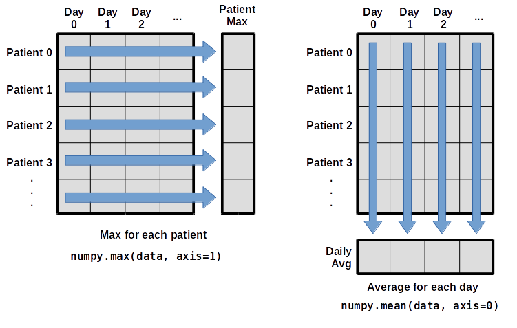
To support this functionality, most array functions allow us to specify the axis we want to work on. If we ask for the average across axis 0 (the rows), we get:

print(numpy.mean(data, axis=0))

[  0.           0.45         1.11666667   1.75         2.43333333   3.15
   3.8          3.88333333   5.23333333   5.51666667   5.95         5.9
   8.35         7.73333333   8.36666667   9.5          9.58333333
  10.63333333  11.56666667  12.35        13.25        11.96666667
  11.03333333  10.16666667  10.           8.66666667   9.15         7.25
   7.33333333   6.58333333   6.06666667   5.95         5.11666667   3.6
   3.3          3.56666667   2.48333333   1.5          1.13333333
   0.56666667]

This is a one-dimensional array, where each entry corresponds to a day, and represents the average inflammation across all patients (rows) for that day.

If we average across axis 1 (columns), we get:

print(numpy.mean(data, axis=1))

[ 5.45   5.425  6.1    5.9    5.55   6.225  5.975  6.65   6.625  6.525
  6.775  5.8    6.225  5.75   5.225  6.3    6.55   5.7    5.85   6.55
  5.775  5.825  6.175  6.1    5.8    6.425  6.05   6.025  6.175  6.55
  6.175  6.35   6.725  6.125  7.075  5.725  5.925  6.15   6.075  5.75
  5.975  5.725  6.3    5.9    6.75   5.925  7.225  6.15   5.95   6.275  5.7
  6.1    6.825  5.975  6.725  5.7    6.25   6.4    7.05   5.9  ]

which is the average inflammation per patient across all days.

Challenge: Calculations on subsets of data

How would you calculate the average inflammation for all patients during the first four days of the trial?

Solution

print(numpy.mean(data[:,0:4]))

0.8291666666666667

The key is the slice data[:,0:4]. We want to include all patients (rows) in the calculation, so we keep every row (: in the x index), but only include the first four days (columns), so we exclude the rest with 0:4 in the y index.

We could also write this slice as data[:,:4].

Keypoints

• Import a library into a program using import libraryname.

• Use the numpy library to work with arrays in Python.

• The expression array.shape gives the shape of an array.

• Use array[x, y] to select a single element from a 2D array.

• Array indices start at 0, not 1.

• Use low:high to specify a slice that includes the indices from low to high-1.

• Use # some kind of explanation to add comments to programs.

• Use numpy.mean(array), numpy.max(array), and numpy.min(array) to calculate simple statistics.

• Use numpy.mean(array, axis=0) or numpy.mean(array, axis=1) to calculate statistics across the specified axis.

---

[1]

Usually, we would have to first install NumPy before we could import it. Here we’re using an environment that comes with NumPy already installed, so we don’t need to.